Refining Vector Search Queries With Time Filters in pgvector: A Tutorial

Vector databases have emerged as a powerful solution for working with high-dimensional data. These databases store vectors and perform vector searches. A vector is an array of numbers representing a data point in a multi-dimensional space, and vector search finds the most similar vectors to a query vector in this space. Vector search capabilities are powerful in machine learning and artificial intelligence, where traditional text-based search falls short.

Refining vector search queries becomes increasingly essential as data grows in volume. This is where time filters come into play. Time-based filtering allows users to narrow search results based on temporal criteria, such as creation date, modification date, or any time-related attribute associated with the data. Whether finding the most recent documents or documents from a specific time range, time-based filtering provides a crucial capability that complements similarity search.

Not all vector databases support both vector search and time-based filtering. The ability to perform both in the database unlocks efficiencies not otherwise possible. PostgreSQL with the pgvector and timescaledb extensions provides a potent platform for combining vector search with time-based filtering using SQL. In this post, we will explore vector search, time-based search, and several approaches to how one might combine the two. We will evaluate the speed and efficiency of these options.

Vector Search Queries With Time Filters: The Roadmap

In this hands-on orientation, we will load a sample dataset into a table and run time-filtered vector search queries against it. We can understand how Postgres executes each vector search query by examining the query plans. Furthermore, we can evaluate the performance of each query.

Here’s an overview of what we’ll cover:

Query plans: First, we will provide a brief description of query plans in Postgres. If you are a seasoned query tuner, skip ahead to the setup.

Setup: In the second section, we will do all our prep work. We will create a Timescale service, create a table, and load it with our sample dataset.

Filtering documents by time: In the next section, we will look at time-based filtering in isolation. We will explore the power of TimescaleDB’s hypertables (which automatically partition Postgres tables into smaller data partitions or chunks) and compare them to plain Postgres tables. Feel free to skip ahead if you are already familiar with hypertables and time-based filtering.

Vector search: After looking at time-based filtering in isolation, we will look at vector search in isolation. This section will introduce the features the pgvector and Timescale Vector extensions provide. You can safely jump past this if you know how to do vector search in Postgres.

Vector search and querying by time: In this section, we will learn how to do both time-based filtering and similarity search in a single SQL query. (When the vectors contain a large language model’s embedding of textual content, vector search is a search of semantic similarity.) We will play with a few different versions of the query and see how Postgres decides to execute them.

Using vector search and time filters in AI applications: Once we’ve covered the techniques for combining vector similarity search and time filters, we’ll briefly explore how to apply what we learned to building GenAI applications.

Query Plans

When discussing query tuning in PostgreSQL, an essential concept to grasp is a "query plan." A query plan is a set of steps the PostgreSQL query planner generates describing how PostgreSQL will execute a SQL query. Various factors, including the query structure, the database schema, and the statistical information about the data distribution in the tables, influence the chosen query plan.

To evaluate a query plan in PostgreSQL, you can use the EXPLAIN command followed by your query. This command returns the planner's chosen execution plan without executing the query. It will show the plan's overall cost and each step's cost. Cost is a unitless measure but can be used to compare the relative performance of one query to another. For a more detailed analysis, including the execution times, you can use EXPLAIN ANALYZE, which executes the query. However, be cautious with EXPLAIN ANALYZE on production systems, as it can affect performance.

Don’t worry! We won’t get too bogged down in the minutia of query plans. We will use EXPLAIN ANALYZE to compare the speed and efficiency of various queries, but we will keep it light.

Note: Because many variables influence query plans, you may see query plans that are not exactly like the ones depicted; however, they should be similar enough to draw the same conclusions.

Another note: If you want to see a visual representation of query plans, there is an excellent, free tool for this at https://explain.dalibo.com/

The Setup

We will load a table with a sample dataset and run queries against it to explore time-based filtering and semantic search. We will use a modified version of the Cohere wikipedia-22-12-simple-embeddings dataset hosted on Huggingface. It contains embeddings of Simple English Wikipedia entries.

We added synthetic data: a time column, category, and tags. We loaded the data into a Postgres table and exported it to a CSV file; therefore, the format has changed. The original dataset on Huggingface is available under the Apache 2.0 license, and thus, our modified version is also subject to the Apache 2.0 license.

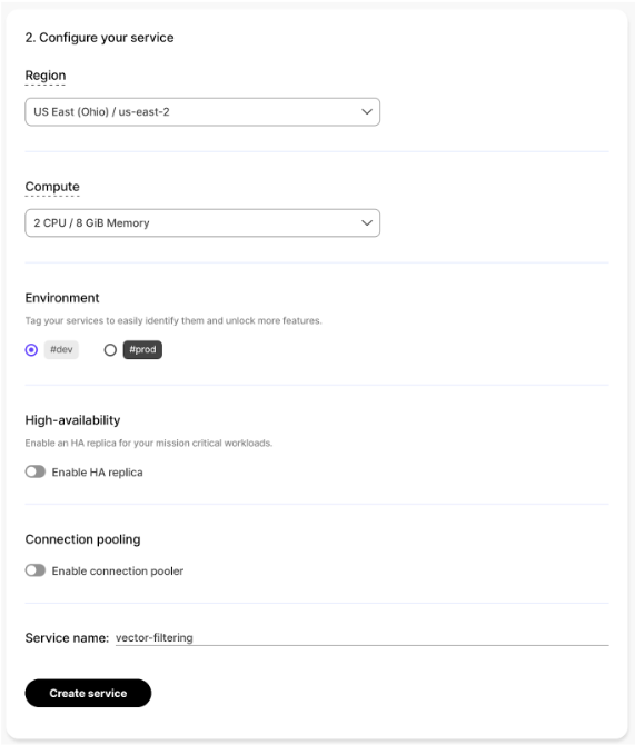
You will need a database if you want to follow along. Head to the Timescale console (you can try Timescale Vector for free with a 90-day extended trial) and create a “Time Series and Analytics” service. Building vector indexes can be a compute-hungry activity, so choose 2 CPU / 8 GiB Memory compute. Choose a region close to you for the best experience.

Image of the page in the Timescale console where you can create a Time Series and Analytics service

We need some sample data to load into our database. The dataset we will use is available on Huggingface. Use this link to download the CSV file.

Make sure you have the psql client installed locally. You will need psql version 16 or greater. Run psql --version to see what version you have.

Connect to your Timescale service using the psql client. Pass the connection URL as an argument. Make sure the wiki.csv file you downloaded is in the same directory where you launch psql.

psql "<connection url>"

We will use three extensions, including timescaledb, pgvector, and timescale_vector. We need to ensure these extensions exist before creating our table.

create extension if not exists timescaledb;
create extension if not exists vector;
create extension if not exists timescale_vector;

Run the following statement to create a table named wiki. The embeddingcolumn is of type vector(768) and will contain our embeddings. The pgvector extension provides the vector type.

create table public.wiki
( id int not null
, time timestamptz not null
, contents text
, meta jsonb
, embedding vector(768)
);

Next, run the following command to convert the plain Postgres table into a TimescaleDB hypertable. The hypertable divides the dataset into day-sized sub-tables called chunks based on the values in the time column.

select create_hypertable
( 'public.wiki'::regclass
, 'time'::name
, chunk_time_interval=>'1d'::interval
);

Now that we have a place to put our data, we can load our data. Run this meta-command to load the data from the CSV file into the wiki table. Expect this to take a few minutes.

\copy wiki from 'wiki.csv' with (format csv, header on)

Make sure Postgres has accurate statistics for our new table. Statistics will influence the query plans.

analyze wiki;

You should find 485,859 rows in the wiki table if you have done this correctly.

select count(*) from wiki;

Finally, let’s turn off parallelism to keep our query plans simple.

set max_parallel_workers_per_gather = 0;

You are ready to go!

Filtering Documents by Time

Our wiki table contains a timestamptz column named time. The data in this column is fake. We have added these timestamps so that we have something to illustrate filtering by time. You would use the timestamp associated with a web page or document in real-world use.

We will use the power of TimescaleDB's hypertables to facilitate filtering by time. A hypertable is a logical table broken up into smaller physical tables called chunks. Each chunk contains data falling within a time range, and the time ranges of the chunks do not overlap. If you are familiar with partitioning or inheritance in Postgres, you can think of hypertables in these terms.

Why is this helpful? When querying a hypertable and filtering on a given time range, TimescaleDB can do chunk exclusion: it ignores any chunks whose time ranges fall outside the bounds of the time range filter, and Postgres expends no compute resources to process the rows in the excluded chunks. Eliminating large chunks of the table through chunk exclusion speeds up time-filtered search.

There are 485,859 rows in the dataset. As we loaded the data, we assigned a date to each row and incremented the date each time we loaded 50,000 rows, giving us 10 chunks. Nine chunks have 50,000 rows, and the last chunk has 35,859. Below are the time range bounds and row counts for the 10 chunks.

┌─────────────┬────────────┬───────┐
│ range_start │ range_end  │ count │
├─────────────┼────────────┼───────┤
│ 2000-01-01  │ 2000-01-02 │ 50000 │
│ 2000-01-02  │ 2000-01-03 │ 50000 │
│ 2000-01-03  │ 2000-01-04 │ 50000 │
│ 2000-01-04  │ 2000-01-05 │ 50000 │
│ 2000-01-05  │ 2000-01-06 │ 50000 │
│ 2000-01-06  │ 2000-01-07 │ 50000 │
│ 2000-01-07  │ 2000-01-08 │ 50000 │
│ 2000-01-08  │ 2000-01-09 │ 50000 │
│ 2000-01-09  │ 2000-01-10 │ 50000 │
│ 2000-01-10  │ 2000-01-11 │ 35859 │
└─────────────┴────────────┴───────┘
(10 rows)

The query below filters the wiki table on a time range. We use explain analyze to get Postgres to run the query and tell us what it did.

explain analyze
select id
from wiki
where '2000-01-04'::timestamptz <= time and time < '2000-01-06'::timestamptz
;

The query plan shows that Postgres did a sequential scan on two chunks of the hypertable. Postgres returned 100,000 rows in total. Postgres excluded the other eight chunks and did not have to expend resources to process the rows in those chunks. Again, chunk exclusion is a hypertable’s superpower; it allows for faster and more efficient queries when filtering on a time range.

QUERY PLAN
Append  (cost=0.00..10064.00 rows=100000 width=4) (actual time=0.005..30.934 rows=100000 loops=1)
  ->  Seq Scan on _hyper_1_4_chunk  (cost=0.00..4846.00 rows=50000 width=4) (actual time=0.005..12.453 rows=50000 loops=1)
        Filter: (('2000-01-04 00:00:00+00'::timestamp with time zone <= "time") AND ("time" < '2000-01-06 00:00:00+00'::timestamp with time zone))
  ->  Seq Scan on _hyper_1_5_chunk  (cost=0.00..4718.00 rows=50000 width=4) (actual time=0.006..12.622 rows=50000 loops=1)
        Filter: (('2000-01-04 00:00:00+00'::timestamp with time zone <= "time") AND ("time" < '2000-01-06 00:00:00+00'::timestamp with time zone))
Planning Time: 0.197 ms
Execution Time: 33.925 ms

To illustrate the savings associated with the chunk exclusion, we can create a wiki2 table exactly like wiki except wiki2 is a plain table—not a hypertable.

Note: the insert will take a minute or two. Be patient.

create table public.wiki2
( id int not null
, time timestamptz not null
, contents text
, meta jsonb
, embedding vector(768)
);

insert into wiki2 select * from wiki;

analyze wiki2;

explain analyze
select id
from wiki2
where '2000-01-04'::timestamptz <= time and time < '2000-01-06'::timestamptz
;

Running the same query against wiki2 gives us the following query plan. Using the plain table is more expensive and slower than using the hypertable. In this case, Postgres had to “look at” all 485,859 rows in the table to find the 100,000 that match the time filter.

QUERY PLAN
Seq Scan on wiki2  (cost=0.00..44853.14 rows=102261 width=4) (actual time=31.259..105.586 rows=100000 loops=1)
  Filter: (('2000-01-04 00:00:00+00'::timestamp with time zone <= "time") AND ("time" < '2000-01-06 00:00:00+00'::timestamp with time zone))
  Rows Removed by Filter: 385859
Planning Time: 0.631 ms
Execution Time: 108.655 ms

You may say this is not a fair comparison because any reasonable developer would put an index on time. Let's try that.

create index on wiki2 (time);

QUERY PLAN
Index Scan using wiki2_time_idx on wiki2  (cost=0.42..10049.55 rows=102257 width=4) (actual time=0.013..26.817 rows=100000 loops=1)
  Index Cond: (("time" >= '2000-01-04 00:00:00+00'::timestamp with time zone) AND ("time" < '2000-01-06 00:00:00+00'::timestamp with time zone))
Planning Time: 0.086 ms
Execution Time: 29.917 ms

┌────────────┬──────────┬────────────┐
│    type    │   cost   │    time    │
├────────────┼──────────┼────────────┤
│ hypertable │ 10064.00 │  33.925 ms │
│ plain      │ 44853.14 │ 108.655 ms │
│ indexed    │ 10049.55 │  29.917 ms │
└────────────┴──────────┴────────────┘

At least for this dataset on this machine type, an indexed plain table is slightly cheaper and faster than a hypertable. So, why would we use a hypertable? There are a couple of reasons. Firstly, as this dataset gets larger, it becomes more likely that the hypertable will outperform the plain table. Secondly, Postgres will use only one index per table per query in most situations. We want to use a hypertable because we are not finished filtering, and we want to use a different index altogether.

Vector Search

As a reminder, we ultimately want to combine time filtering and vector search. Let's explore vector search in isolation first. If you are already a confident user of similarity search with pgvector, feel free to jump ahead.

Our wiki table has a column named embedding of type vector(768). The pgvector extension provides the vector datatype. This column contains the embeddings of the wiki content.

We will grab a random vector to use as a search parameter. The psql client makes this easy. We can select the embedding column from a row and use the \gset meta-command to create a variable in the psql client named emb containing the vector value. We can use this variable as a parameter for future queries. In this case, we will use the vector from the row with id 65272. In subsequent queries, we will search for rows where the embedding is semantically similar to the row with id 65272.

select embedding as emb
from wiki
where id = 65272
\gset

Next, we query the wiki table and use the <=> (cosine) distance operator provided by pgvector and timescale_vector. This operator computes the distance between two vectors, and this distance is a representation of how semantically similar the two vectors are. If we order by the similarity distance and limit the results to 10, our query will return the 10 rows most semantically similar to the content from row 65272.

Note: The $1 in the query below denotes a query parameter, and the \bind meta-command assigns the value from our emb psql variable to this parameter.

select id, embedding <=> $1::vector as dist
from wiki
order by dist
limit 10
\bind :emb
;

┌────────┬─────────────────────┐
│   id   │        dist         │
├────────┼─────────────────────┤
│  65272 │                   0 │
│  16295 │  0.1115766717013853 │
│  16302 │ 0.11360477414644143 │
│  16297 │ 0.12387882580027065 │
│  16298 │  0.1299166956232466 │
│  34598 │ 0.13121629452715455 │
│  16292 │ 0.13307570937651947 │
│  61078 │ 0.13427528064358674 │
│ 215163 │ 0.13759063950532036 │
│  79614 │ 0.13770102915039784 │
└────────┴─────────────────────┘
(10 rows)

As expected, row 65272 is the top result with exactly the vector we borrowed for the query. Nine more results follow with increasing distance.

Looking at the query plan for this, we find that Postgres scanned the entire table and performed the distance calculation on the fly for each of the 485,859 rows. This execution took 3,441 milliseconds, considerably longer than any time-based filtering approaches we had previously explored.

explain analyze
select id, embedding <=> $1::vector as dist
from wiki
order by dist
limit 10
\bind :emb
;

QUERY PLAN
Limit  (cost=62004.36..62004.39 rows=10 width=12) (actual time=3440.996..3441.002 rows=10 loops=1)
  ->  Sort  (cost=62004.36..63219.01 rows=485859 width=12) (actual time=3440.994..3441.000 rows=10 loops=1)
        Sort Key: ((_hyper_1_1_chunk.embedding <=> '[...]'::vector))
        Sort Method: top-N heapsort  Memory: 25kB
        ->  Result  (cost=0.00..51505.12 rows=485859 width=12) (actual time=0.030..3357.861 rows=485859 loops=1)
              ->  Append  (cost=0.00..45431.88 rows=485859 width=22) (actual time=0.015..329.158 rows=485859 loops=1)
                    ->  Seq Scan on _hyper_1_1_chunk  (cost=0.00..4788.00 rows=50000 width=22) (actual time=0.015..30.596 rows=50000 loops=1)
                    ->  Seq Scan on _hyper_1_2_chunk  (cost=0.00..4724.00 rows=50000 width=22) (actual time=0.013..31.533 rows=50000 loops=1)
                    ->  Seq Scan on _hyper_1_3_chunk  (cost=0.00..4660.00 rows=50000 width=22) (actual time=0.012..31.167 rows=50000 loops=1)
                    ->  Seq Scan on _hyper_1_4_chunk  (cost=0.00..4596.00 rows=50000 width=22) (actual time=0.012..30.917 rows=50000 loops=1)
                    ->  Seq Scan on _hyper_1_5_chunk  (cost=0.00..4468.00 rows=50000 width=22) (actual time=0.013..29.304 rows=50000 loops=1)
                    ->  Seq Scan on _hyper_1_6_chunk  (cost=0.00..4340.00 rows=50000 width=22) (actual time=0.012..28.831 rows=50000 loops=1)
                    ->  Seq Scan on _hyper_1_7_chunk  (cost=0.00..4276.00 rows=50000 width=22) (actual time=0.012..29.065 rows=50000 loops=1)
                    ->  Seq Scan on _hyper_1_8_chunk  (cost=0.00..4148.00 rows=50000 width=22) (actual time=0.013..28.186 rows=50000 loops=1)
                    ->  Seq Scan on _hyper_1_9_chunk  (cost=0.00..3956.00 rows=50000 width=22) (actual time=0.012..27.490 rows=50000 loops=1)
                    ->  Seq Scan on _hyper_1_10_chunk  (cost=0.00..3046.59 rows=35859 width=22) (actual time=0.011..20.635 rows=35859 loops=1)
Planning Time: 0.231 ms
Execution Time: 3441.034 ms

Can we make vector search faster and cheaper? Yes, we can do it by using an index. The pgvector extension provides two types of indexes: ivfflat and hnsw. The timescale_vector extension provides a third: tsv. All three index types implement approximate nearest-neighbor search algorithms. None of them will produce exact results, but they will make our searches considerably more efficient. As the number of vectors grows past a certain scale, exact searches become impractical.

This tutorial will use the tsv index type and its default settings.

Note: Expect creating the index to take 10 minutes or more.

create index on wiki using tsv (embedding);

You will note that we get slightly different results when we execute the same query. Without the index, Postgres performs an exhaustive and exact search. With the index, Postgres performs an approximate search. We trade some measure of accuracy for speed and efficiency. We can see how fast and efficient it is by looking at the query plan.

select id, embedding <=> $1::vector as dist
from wiki
order by dist
limit 10
\bind :emb
;

┌───────┬─────────────────────┐
│  id   │        dist         │
├───────┼─────────────────────┤
│ 65272 │                   0 │
│ 16302 │ 0.11360477414644143 │
│ 16295 │  0.1115766717013853 │
│ 16297 │ 0.12387882580027065 │
│ 16298 │  0.1299166956232466 │
│ 34598 │ 0.13121629452715455 │
│ 16292 │ 0.13307570937651947 │
│ 61078 │ 0.13427528064358674 │
│ 79614 │ 0.13770102915039784 │
│ 16307 │  0.1408329687219958 │
└───────┴─────────────────────┘
(10 rows)

The query plan shows that the query cost 2720.81 and took 24.642 milliseconds to execute. The version of the query that did not use the index cost 62004.39 and took 3441.034 milliseconds. The index made a huge difference! Instead of doing a sequential scan on all the chunks, Postgres did an index scan on each chunk.

QUERY PLAN
Limit  (cost=2719.51..2720.81 rows=10 width=12) (actual time=24.317..24.578 rows=10 loops=1)
  ->  Result  (cost=2719.51..66108.97 rows=485859 width=12) (actual time=24.316..24.575 rows=10 loops=1)
        ->  Merge Append  (cost=2719.51..60035.73 rows=485859 width=22) (actual time=24.315..24.572 rows=10 loops=1)
              Sort Key: ((_hyper_1_1_chunk.embedding <=> '[...]'::vector))
              ->  Index Scan using _hyper_1_1_chunk_wiki_embedding_idx on _hyper_1_1_chunk  (cost=279.85..5496.65 rows=50000 width=22) (actual time=1.846..1.982 rows=7 loops=1)
                    Order By: (embedding <=> '[...]'::vector)
              ->  Index Scan using _hyper_1_2_chunk_wiki_embedding_idx on _hyper_1_2_chunk  (cost=279.85..5426.25 rows=50000 width=22) (actual time=2.247..2.361 rows=4 loops=1)
                    Order By: (embedding <=> '[...]'::vector)
              ->  Index Scan using _hyper_1_3_chunk_wiki_embedding_idx on _hyper_1_3_chunk  (cost=279.85..5355.85 rows=50000 width=22) (actual time=2.327..2.327 rows=1 loops=1)
                    Order By: (embedding <=> '[...]'::vector)
              ->  Index Scan using _hyper_1_4_chunk_wiki_embedding_idx on _hyper_1_4_chunk  (cost=279.85..5285.45 rows=50000 width=22) (actual time=2.265..2.265 rows=1 loops=1)
                    Order By: (embedding <=> '[...]'::vector)
              ->  Index Scan using _hyper_1_5_chunk_wiki_embedding_idx on _hyper_1_5_chunk  (cost=279.85..5144.65 rows=50000 width=22) (actual time=2.849..2.849 rows=1 loops=1)
                    Order By: (embedding <=> '[...]'::vector)
              ->  Index Scan using _hyper_1_6_chunk_wiki_embedding_idx on _hyper_1_6_chunk  (cost=279.85..5003.85 rows=50000 width=22) (actual time=2.625..2.625 rows=1 loops=1)
                    Order By: (embedding <=> '[...]'::vector)
              ->  Index Scan using _hyper_1_7_chunk_wiki_embedding_idx on _hyper_1_7_chunk  (cost=279.85..4933.45 rows=50000 width=22) (actual time=2.805..2.805 rows=1 loops=1)
                    Order By: (embedding <=> '[...]'::vector)
              ->  Index Scan using _hyper_1_8_chunk_wiki_embedding_idx on _hyper_1_8_chunk  (cost=279.85..4792.65 rows=50000 width=22) (actual time=2.496..2.497 rows=1 loops=1)
                    Order By: (embedding <=> '[...]'::vector)
              ->  Index Scan using _hyper_1_9_chunk_wiki_embedding_idx on _hyper_1_9_chunk  (cost=279.85..4581.45 rows=50000 width=22) (actual time=2.160..2.161 rows=1 loops=1)
                    Order By: (embedding <=> '[...]'::vector)
              ->  Index Scan using _hyper_1_10_chunk_wiki_embedding_idx on _hyper_1_10_chunk  (cost=200.69..3516.08 rows=35859 width=22) (actual time=2.689..2.689 rows=1 loops=1)
                    Order By: (embedding <=> '[...]'::vector)
Planning Time: 0.288 ms
Execution Time: 24.642 ms

Notice that we got different results from the two queries. The version without the index had to calculate the exact distances on the fly—a big part of its slowness. The indexed version used an approximate nearest-neighbor algorithm. Its results were not exact, but they were delivered faster and cheaper.

Vector Search and Filtering by Time

Now that we have explored filtering by time and vector search in isolation, can we combine the two in a single efficient query?

select id, embedding <=> $1::vector as dist
from wiki
where '2000-01-02'::timestamptz <= time and time < '2000-01-04'::timestamptz
order by dist
limit 10
\bind :emb
;

Note: Notice that our results are "worse" in terms of semantic similarity because our time filter has eliminated some of the most similar rows. This outcome is expected. Instead, we have more relevant rows as we excluded rows with high similarity outside our time period of interest.

┌────────┬─────────────────────┐
│   id   │        dist         │
├────────┼─────────────────────┤
│  65272 │                   0 │
│  61078 │ 0.13427528064358674 │
│  79614 │ 0.13770102915039784 │
│  79612 │ 0.14383225467703376 │
│  61080 │  0.1444315737261198 │
│  52634 │  0.1436081460507892 │
│  64473 │ 0.14383654656162292 │
│  61079 │  0.1474735568613179 │
│ 131920 │ 0.15066526846960182 │
│  64475 │   0.154294958183531 │
└────────┴─────────────────────┘
(10 rows)

The query plan reveals that Postgres only considers the two chunks that match the time filter and uses the tsv vector indexes associated with those chunks. We have the best of both worlds!

QUERY PLAN
Limit  (cost=559.71..561.01 rows=10 width=12) (actual time=4.631..5.025 rows=10 loops=1)
  ->  Result  (cost=559.71..13532.11 rows=100000 width=12) (actual time=4.630..5.023 rows=10 loops=1)
        ->  Merge Append  (cost=559.71..12282.11 rows=100000 width=22) (actual time=4.628..5.019 rows=10 loops=1)
              Sort Key: ((_hyper_1_2_chunk.embedding <=> '[...]'::vector))
              ->  Index Scan using _hyper_1_2_chunk_wiki_embedding_idx on _hyper_1_2_chunk  (cost=279.85..5676.25 rows=50000 width=22) (actual time=2.349..2.682 rows=9 loops=1)
                    Order By: (embedding <=> '[...]'::vector)
                    Filter: (('2000-01-02 00:00:00+00'::timestamp with time zone <= "time") AND ("time" < '2000-01-04 00:00:00+00'::timestamp with time zone))
              ->  Index Scan using _hyper_1_3_chunk_wiki_embedding_idx on _hyper_1_3_chunk  (cost=279.85..5605.85 rows=50000 width=22) (actual time=2.277..2.334 rows=2 loops=1)
                    Order By: (embedding <=> '[...]'::vector)
                    Filter: (('2000-01-02 00:00:00+00'::timestamp with time zone <= "time") AND ("time" < '2000-01-04 00:00:00+00'::timestamp with time zone))
Planning Time: 0.257 ms
Execution Time: 5.056 ms

Could we have achieved the same with the indexed plain table? Let's add a tsv index to wiki2 and find out.

Note: Expect creating the index to take 15 minutes or more.

create index on wiki2 using tsv (embedding);

explain analyze
select id, embedding <=> $1::vector as dist
from wiki2
where '2000-01-04'::timestamptz <= time and time < '2000-01-06'::timestamptz
order by dist
limit 10
\bind :emb
;

In most situations, Postgres can only use one index per table at a time. At least in this specific example on this machine, it chooses to use the vector index on embedding. It then filters the time on the fly. If you run this, you may get the same result, or Postgres may choose to do an index scan on the time column to filter by time and then do on-the-fly distance calculations on the vectors.

In this case, the query is as fast as the hypertable approach but nearly five times more expensive. Crucially, as the dataset grows, the hypertable version will increasingly outperform the plain-table version because the hypertable will use chunk exclusion.

QUERY PLAN
Limit  (cost=2709.44..2714.22 rows=10 width=12) (actual time=3.029..5.078 rows=10 loops=1)
  ->  Index Scan using wiki2_embedding_idx on wiki2  (cost=2709.44..51574.47 rows=102257 width=12) (actual time=3.028..5.074 rows=10 loops=1)
        Order By: (embedding <=> '[...]'::vector)
        Filter: (('2000-01-04 00:00:00+00'::timestamp with time zone <= "time") AND ("time" < '2000-01-06 00:00:00+00'::timestamp with time zone))
        Rows Removed by Filter: 73
Planning Time: 0.093 ms
Execution Time: 5.096 ms

Other approaches that did not perform as well.

Can we force Postgres to use both indexes on one plain table? Yes! We can use a subquery. We will order by the vector distance using the vector index in the subquery. In the outer query, we will filter on time using the index on the time column. By joining the two, we will only get results that match both criteria. In other words, querying this way creates two resultsets—one via each index—and these resultsets are then evaluated for intersection.

Note: Technically, we cannot force Postgres to choose to use indexes. Postgres does not have query hints. However, the structure of a query influences the plan. By restructuring the query, we can politely suggest the plan we want.

explain analyze
select w.id, x.dist
from wiki2 w
inner join
(
  select id, embedding <=> $1::vector as dist
  from wiki2
  order by dist
  limit 10
) x on (w.id = x.id)
where '2000-01-02'::timestamptz <= time and time < '2000-01-04'::timestamptz
order by x.dist
\bind :emb
;

QUERY PLAN
Sort  (cost=12868.26..12868.27 rows=2 width=12) (actual time=36.700..36.703 rows=3 loops=1)
  Sort Key: x.dist
  Sort Method: quicksort  Memory: 25kB
  ->  Hash Join  (cost=2711.06..12868.25 rows=2 width=12) (actual time=5.720..36.693 rows=3 loops=1)
        Hash Cond: (w.id = x.id)
        ->  Index Scan using wiki2_time_idx on wiki2 w  (cost=0.42..9784.27 rows=99553 width=4) (actual time=0.013..25.961 rows=100000 loops=1)
              Index Cond: (("time" >= '2000-01-02 00:00:00+00'::timestamp with time zone) AND ("time" < '2000-01-04 00:00:00+00'::timestamp with time zone))
        ->  Hash  (cost=2710.51..2710.51 rows=10 width=12) (actual time=3.111..3.112 rows=10 loops=1)
              Buckets: 1024  Batches: 1  Memory Usage: 9kB
              ->  Subquery Scan on x  (cost=2709.44..2710.51 rows=10 width=12) (actual time=2.693..3.096 rows=10 loops=1)
                    ->  Limit  (cost=2709.44..2710.41 rows=10 width=12) (actual time=2.692..3.092 rows=10 loops=1)
                          ->  Index Scan using wiki2_embedding_idx on wiki2  (cost=2709.44..50104.18 rows=485859 width=12) (actual time=2.690..3.089 rows=10 loops=1)
                                Order By: (embedding <=> '[...]'::vector)
Planning Time: 0.258 ms
Execution Time: 36.737 ms

The query plan shows us that Postgres used both indexes. Surprisingly, having Postgres use both indexes is slower and more costly than both previous approaches. While the subquery only returns 10 rows, the outer query returns 100,000. Postgres then has to evaluate each of the 100,000 rows against each of the 10 rows using a hash join. Returning the 100,000 and comparing them to the 10 is where the bulk of the execution time takes place.

┌───────┬─────────────────────┐
│  id   │        dist         │
├───────┼─────────────────────┤
│ 65272 │                   0 │
│ 61078 │ 0.13427528064358674 │
│ 79614 │ 0.13770102915039784 │
└───────┴─────────────────────┘
(3 rows)

More importantly, we only get three results using the two-index approach. Why is this the case? The vector search subquery considers all the rows regardless of time. It returns the 10 most similar rows from the whole dataset. Unfortunately, seven of these 10 fall outside the time range we are filtering on and, therefore, get excluded from the results. This effect illustrates the classic post-filtering problem common in vector search use cases. Filtering by time after a similarity search can leave you with fewer results than expected or even none at all.

What happens if we turn this query “inside out”? We can put the time filtering in a subquery and do the vector search in the outer query like so:

explain analyze
select w.id, w.embedding <=> $1::vector as dist
from wiki2 w
where exists
(
  select 1
  from wiki2 x
  where '2000-01-02'::timestamptz <= x.time and x.time < '2000-01-04'::timestamptz
  and w.id = x.id
)
order by dist
limit 10
\bind :emb
;

┌────────┬─────────────────────┐
│   id   │        dist         │
├────────┼─────────────────────┤
│  65272 │                   0 │
│  61078 │ 0.13427528064358674 │
│  79614 │ 0.13770102915039784 │
│  52634 │  0.1436081460507892 │
│  79612 │ 0.14383225467703376 │
│  64473 │ 0.14383654656162292 │
│  61080 │  0.1444315737261198 │
│  61079 │  0.1474735568613179 │
│ 131920 │ 0.15066526846960182 │
│  64475 │   0.154294958183531 │
└────────┴─────────────────────┘
(10 rows)

QUERY PLAN
Limit  (cost=58235.37..58235.39 rows=10 width=12) (actual time=1394.904..1394.909 rows=10 loops=1)
  ->  Sort  (cost=58235.37..58484.25 rows=99553 width=12) (actual time=1394.902..1394.906 rows=10 loops=1)
        Sort Key: ((w.embedding <=> '[...]'::vector))
        Sort Method: top-N heapsort  Memory: 25kB
        ->  Hash Semi Join  (cost=11028.68..56084.06 rows=99553 width=12) (actual time=294.332..1380.233 rows=100000 loops=1)
              Hash Cond: (w.id = x.id)
              ->  Seq Scan on wiki2 w  (cost=0.00..42423.59 rows=485859 width=22) (actual time=0.034..616.130 rows=485859 loops=1)
              ->  Hash  (cost=9784.27..9784.27 rows=99553 width=4) (actual time=40.376..40.378 rows=100000 loops=1)
                    Buckets: 131072  Batches: 1  Memory Usage: 4540kB
                    ->  Index Scan using wiki2_time_idx on wiki2 x  (cost=0.42..9784.27 rows=99553 width=4) (actual time=0.016..28.235 rows=100000 loops=1)
                          Index Cond: (("time" >= '2000-01-02 00:00:00+00'::timestamp with time zone) AND ("time" < '2000-01-04 00:00:00+00'::timestamp with time zone))
Planning Time: 0.164 ms
Execution Time: 1394.960 ms

Unfortunately, Postgres used the index on time but chose to ignore the vector index. It computed the exact distances on the fly instead of using an approximate nearest-neighbor search. Unsurprisingly, this approach is slower and more expensive than the single index query plan on the plain table. It is also much slower and more costly than the hypertable approach.

Using Vector Search and Time Filters in AI Applications

Incorporating time-based filtering with semantic search allows AI applications to offer users a more nuanced, context-aware interaction. This approach ensures that the information, products, or content presented is not just relevant but also timely, providing a more valuable user experience.

Content discovery platforms: Imagine a streaming service that not only recommends movies based on your viewing history but also prioritizes new releases or timely content, such as holiday-themed movies. By applying time filters to semantic search, these platforms can dynamically adjust recommendations, ensuring users are presented with content that's not just relevant to their interests but also their recent viewing history or seasonal trends.
News aggregation: Time-based filtering can revolutionize how readers engage with information in news and content aggregation. Time filters can prioritize the latest news, ensuring readers can access the most current information and trends relevant to their query, while semantic search simultaneously sifts through the articles to find ones related to a user's interests.
E-commerce: For e-commerce platforms, combining semantic search with time-based filters can enhance shopping experiences by promoting products related to a user’s recent purchases, upcoming events, or seasonal trends. For instance, suggesting winter sports gear as the season approaches or highlighting flash sale items within a limited time frame makes the shopping experience more relevant and timely.
Academic research: Researchers often seek their field's most recent studies or articles. By integrating time filters with semantic search, academic databases can provide search results that are contextually relevant and prioritize the latest research, facilitating access to cutting-edge knowledge and discoveries.

Next Steps

So, what have we learned? We can combine vector search with time-based filtering in Postgres to retrieve more temporally relevant vectors. While we can achieve this with a plain table, we can write simpler, faster, and more efficient queries that continue to perform as your dataset grows using TimescaleDB’s hypertables.

Use pgvector on Timescale today! Follow this link to get a 90-day free trial!

Ingest and query in milliseconds, even at terabyte scale.

This post was written by