How We Made Real-Time Data Aggregation in Postgres Faster by 50,000%
Hi, we’re Timescale! We build a faster PostgreSQL for demanding workloads like time series, vector, events, and analytics data. Check us out.

Many PostgreSQL users come across materialized views when attempting to speed up their queries through data aggregation. While PostgreSQL materialized views function similarly to query aliases by storing results on disk for faster query performance, they can quickly become outdated. As a result, manual refreshing—accomplished via REFRESH MATERIALIZED VIEW [materialized view name];—is necessary whenever new data is inserted, deleted, or updated in the database to maintain their accuracy.
Having built TimescaleDB on PostgreSQL, we devised a feature to prevent developers from dealing with this challenge: continuous aggregates (CAggs). A core feature of TimescaleDB, continuous aggregates allow the user to pre-compute and speed up aggregation queries over time-series data. They can be seen as a self-updating materialized view, and since TimescaleDB version 1.7, they can do it in real time.
Real-time continuous aggregates allow the computation of results for newly inserted data on the fly. The data is immediately contained in queries that read data from a real-time CAgg, even if the CAgg was not refreshed recently. However, when handling large datasets, we noticed a problem with slow queries, as PostgreSQL needed a lot of time to plan the query. In this blog post, we detail the enhancements made in TimescaleDB 2.13.0 to significantly accelerate real-time data aggregation, resulting in a planning time reduction of over 50,000% and a substantial decrease in query execution times.
Speeding Up Data Aggregation in Postgres: Continuous Aggregates?
To give you a clearer picture of our optimization, let's quickly run through the fundamentals of continuous aggregates. Simply put, a continuous aggregate is like a self-updating materialized view optimized for aggregation queries. Instead of computing the data aggregation from scratch, queries can tap into the CAgg's pre-calculated data, making them zip through the process much faster. Plus, a refresh policy keeps the data up-to-date as and when required.
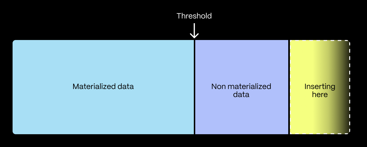
A real-time continuous aggregate consists of (1) materialized data and (2) non-materialized data. The materialized data contains the pre-computed data, whereas the non-materialized data contains the data inserted since the CAgg was refreshed the last time.
These two parts of the CAgg are separated by a threshold value, which we also call the real-time watermark threshold (the watermark for short). When you run a query, and a real-time CAgg is involved, both parts are combined transparently. The pre-computed data is read from the materialized part, and the real-time part is computed on the fly.
The pre-computed data is stored in a hypertable (a regular PostgreSQL table that automatically partitions data), which is called the materialized hypertable. In contrast, we denote the input hypertable and the raw hypertable to distinguish between these two hypertables.
Since a continuous aggregate is implemented as a specialized materialized view in PostgreSQL, the \d+ command
in psql can be used to get the underlying query of the continuous aggregate.
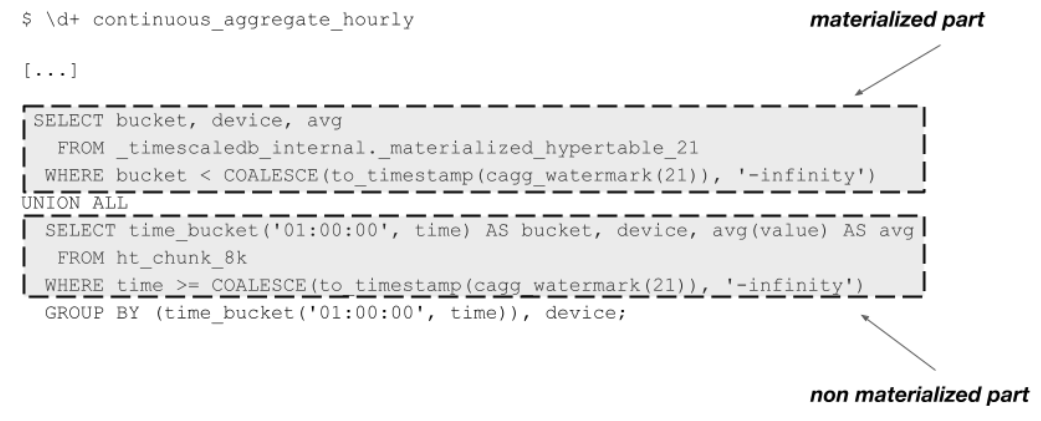
The query consists of two parts that follow the structure of the real-time continuous aggregates: one part queries the materialized part of the continuous aggregate, and the other queries the non-materialized part and calculates the results on demand. Both parts of the query are combined using a UNION operation.
Query Planning in Postgres and Function Volatility
Before we deep dive into the changes we introduced to our code base, let’s first discuss some basics about query planning and function volatility in PostgreSQL.
A query plan needs to be computed to execute a query in PostgreSQL. The query only describes how the result should look like. However, to execute a query, PostgreSQL needs to know which operators (e.g., filters, join) and input data (e.g., a table scan or an index scan) have to be used to produce the desired query result. So, the query plan contains the exact information on which steps are needed to execute the query.
There are several ways to compute a query. However, one might be more efficient than the other. For example, when the following query is executed: SELECT * FROM customer WHERE lastname = upper('Smith'); and an index on the column lastname exists, there are at least two ways to execute the query:
- Perform a full table scan and evaluate the predicate on every row—execute the
upper()function and check if thelastnameattribute is equal to this result. - Execute the
upper()function and perform an index scan to fetch only the needed tuples.
The index scan might be the more performant alternative, especially when it comes to large relations. Internally, PostgreSQL considered both plans, annotated them with costs, and chose the cheapest plan. This method of determining the optimal plan is called cost-based optimization in database systems.
An important question in this example is, is PostgreSQL allowed to execute the upper function during query planning and use the result to create an index scan? This depends on the function volatility type. In our example, the upper() function always returns the same result for the same input (i.e., if we input Smith, the output will always be SMITH). However, if we have a function that returns a random value, it always returns a different value.
PostgreSQL uses the following volatility classifications to distinguish the behavior of functions:
- VOLATILE: These functions can return different values for the same arguments. So, the result of the function call cannot be cached.
- STABLE: These functions return the same result for the same argument within a single statement. PostgreSQL can replace multiple invocations of the same function with a single invocation.
- IMMUTABLE: These functions always return the same result for the same input. So, the function can be pre-evaluated during query planning, and the function invocation by a constant value in the query plan.
Since the upper() function is marked as STABLE, PostgreSQL can replace its invocation during planning time with a constant and construct the index scan, as mentioned earlier.
Example
In this example, we create a table with the name test that contains 1,000,000 tuples. The table consists only of one attribute, which is also marked as the primary key. Therefore, an index is also automatically created for this attribute.
In the next step, a function named one() is defined, which returns an integer value of 50,000. This function is used in the following steps with different volatility classes to illustrate how PostgreSQL evaluates it.
test=# CREATE TABLE test(i INTEGER PRIMARY KEY);
INSERT INTO test SELECT generate_series(1,1000000);
VACUUM ANALYZE test;
CREATE TABLE
INSERT 0 1000000
VACUUM
test=# CREATE FUNCTION one() RETURNS INTEGER
LANGUAGE plpgsql
AS 'BEGIN RETURN 500000; END;';
CREATE FUNCTION
We will use the function in the following query SELECT * FROM test WHERE i = one();. The idea of the query is to find the record whose attribute i is equal to 50,000. However, due to the different volatility classes, PostgreSQL can perform different optimizations and the generated query plan changes.
Function volatility VOLATILE
When the function is marked as volatile, PostgreSQL can not optimize the function since it claims the result can change on each invocation. The query plans show that a sequential scan is used, and the scan removes 999,999 of the scanned tuples.
test=# ALTER FUNCTION one() VOLATILE;
ALTER FUNCTION
test=# EXPLAIN (ANALYZE) SELECT * FROM test WHERE i = one();
                                                 QUERY PLAN
------------------------------------------------------------------------------------------------------------
 Seq Scan on test  (cost=0.00..266925.00 rows=1 width=4) (actual time=509.934..1051.636 rows=1 loops=1)
   Filter: (i = one())
   Rows Removed by Filter: 999999
 Planning Time: 0.426 ms
 JIT:
   Functions: 2
   Options: Inlining false, Optimization false, Expressions true, Deforming true
   Timing: Generation 0.080 ms, Inlining 0.000 ms, Optimization 0.087 ms, Emission 1.331 ms, Total 1.497 ms
 Execution Time: 1063.245 ms
(9 rows)
Function volatility STABLE
In the second example, the function volatility is changed to STABLE. Therefore, PostgreSQL is allowed to replace multiple function invocations with the same parameter (i.e., the empty parameter in our example) in a single statement with a single execution of the function at execution time.
Since the function result is known to be the same, an index operation can be used to find the desired record. PostgreSQL is allowed to evaluate the function one time during query execution and use the result to perform the index access. This is shown in the following query plan: an index scan replaces the sequential scan with the condition i = one(). Since an index scan is used, the query execution is much more efficient. Only the desired record is fetched from the table.
test=# ALTER FUNCTION one() STABLE;
ALTER FUNCTION
test=# EXPLAIN (ANALYZE) SELECT * FROM test WHERE i = one();
                                                     QUERY PLAN
---------------------------------------------------------------------------------------------------------------------
 Index Only Scan using test_pkey on test  (cost=0.68..4.69 rows=1 width=4) (actual time=0.060..0.063 rows=1 loops=1)
   Index Cond: (i = one())
   Heap Fetches: 0
 Planning Time: 0.472 ms
 Execution Time: 0.126 ms
(5 rows)
Function volatility IMMUTABLE
In the last example, the function is now classified as IMMUTABLE. Therefore, PostgreSQL is allowed to evaluate the function during query planning and replace it with a constant value. This is exactly what happened in the following query plan; the condition of the index was changed from i = one() to i = 50000:
test=# ALTER FUNCTION one() IMMUTABLE;
ALTER FUNCTION
test=# EXPLAIN (ANALYZE) SELECT * FROM test WHERE i = one();
                                                     QUERY PLAN
---------------------------------------------------------------------------------------------------------------------
 Index Only Scan using test_pkey on test  (cost=0.42..4.44 rows=1 width=4) (actual time=0.046..0.049 rows=1 loops=1)
   Index Cond: (i = 500000)
   Heap Fetches: 0
 Planning Time: 0.397 ms
 Execution Time: 0.102 ms
(5 rows)
The function volatility of the watermark function
What does all of this have to do with real-time CAggs? The watermark value of the real-time CAgg, which indicates which data has the read from the materialized hypertable and which data needs to be computed on the fly, is exposed in the queries via the _timescaledb_functions.cagg_watermark() function. The function takes the ID of the materialized hypertable and returns the current watermark value for this continuous aggregate.
The watermark value changes when the CAgg changes. When new data is added to the raw hypertable and the CAgg is updated, it moves forward in time. When data is deleted from the raw hypertable and the CAgg is refreshed, the watermark might go backward (this depends on whether the refresh actually deletes data or is not performed for this time interval, keeping the data in the CAgg). Since the watermark function can return different values for the same input parameter, the function is declared as STABLE.
Query Planning When a Real-Time Continuous Aggregate Is Used
Unfortunately, real-time CAggs performed slower than expected in some cases. This is especially true for large data sets with many chunks. Surprisingly, the execution of the real-time part is the cause of the slow performance. The query planning contributes the most significant part of the time that is needed to process the SQL query.
The reason for this is the volatility classification of the _timescaledb_functions.cagg_watermark() function. Because it is marked as STABLE, PostgreSQL could not evaluate the function at planning time. Therefore, it is unknown to the planner which chunks need to be scanned using the real-time part of the query and which parts need to be handled by the materialized part of the query. As a consequence, PostgreSQL needs to plan for the worst case and needs to plan a real-time scan for all chunks.
The following EXPLAIN output shows a shortened version of the query plan for a SELECT query on a continuous aggregate. The query plans show that the index scan invokes the _timescaledb_functions.cagg_watermark() function and that the function result is not pre-evaluated at planning time.
HashAggregate (actual rows=4 loops=1)
  Group Key: time_bucket(10, boundary_test."time")
  Group Key: time_bucket(10, _hyper_5_5_chunk."time")
  Batches: 1
  ->  Result (actual rows=4 loops=1)
        ->  Custom Scan (ChunkAppend) on boundary_test (actual rows=4 loops=1)
              Chunks excluded during startup: 0
        ->  Append (actual rows=4 loops=1)
              ->  Index Scan Backward using _hyper_5_5_chunk_boundary_test_time_idx on _hyper_5_5_chunk (actual rows=1 loops=1)
                    Index Cond: ("time" >= COALESCE((_timescaledb_functions.cagg_watermark(6))::integer, '-2147483648'::integer))
              ->  Index Scan Backward using _hyper_5_6_chunk_boundary_test_time_idx on _hyper_5_6_chunk (actual rows=1 loops=1)
                    Index Cond: ("time" >= COALESCE((_timescaledb_functions.cagg_watermark(6))::integer, '-2147483648'::integer))
       -> [...]
Especially on large hypertables, query planning takes a significant amount of time. We experimented with a hypertable with 8,000 chunks to understand the behavior better. The planning time for a regular continuous aggregate took 227.874 ms. However, the planning time increased to more than two minutes after activating the CAgg's real-time feature.
To better understand PostgreSQL's behavior, we used a profiler to identify where additional time is spent in the code. A profiler periodically samples a running program and stores information on which part of the code is executed. Code parts that require a lot of time are more often sampled by the profiler than code paths that are only executed rarely.
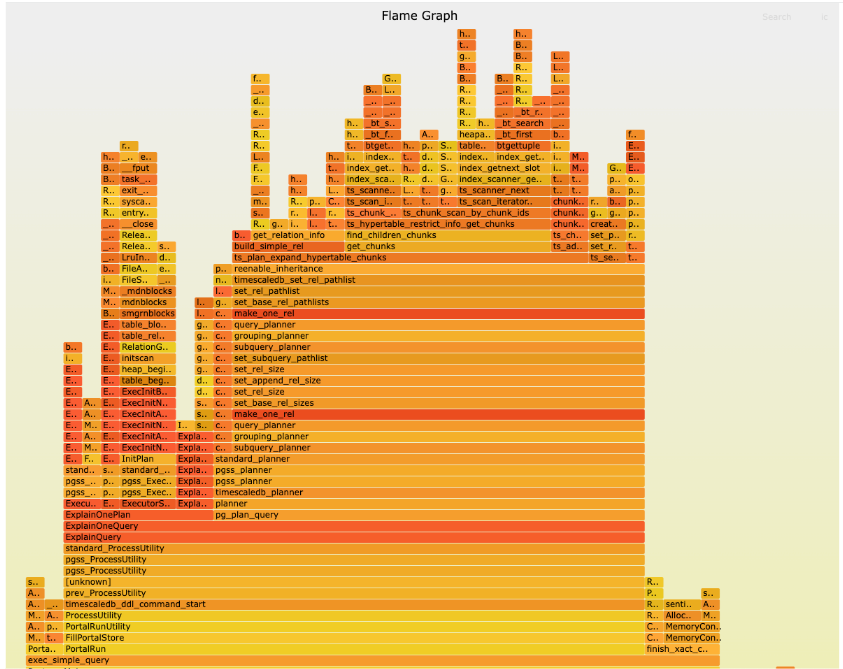
Flame graphs are a common technique for visualizing the output. They aggregate the profiler's output in a graphical way for easy analysis.
“Flame graphs are a visualization of hierarchical data, created to visualize stack traces of profiled software so that the most frequent code-paths to be identified quickly and accurately.”
The following flame graph is based on the samples from executing a SELECT query on our CAgg with 8,000 chunks.
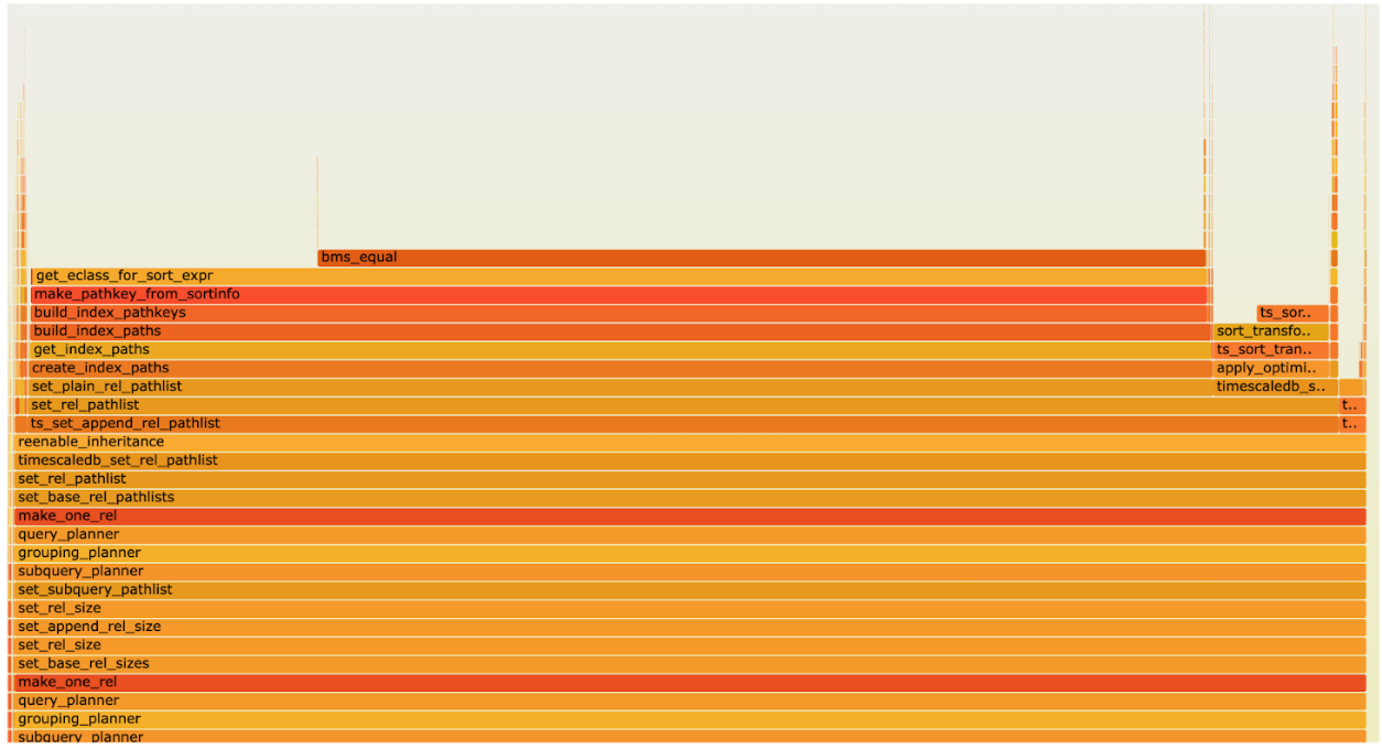
The flame graph shows that PostgreSQL spends a lot of time finding equivalence class members and the bms_equal() function is called very often when the index scan paths are created. The reason for this is a shortcoming of PostgreSQL when index scans on partitioned tables are planned.
To speed up the planning for real-time continuous aggregates, it might be beneficial to plan only scans for the chunks that are actually accessed by the query. However, this requires information about the watermark value at plan time. Unfortunately, the information is unknown due to the volatility of the function.
Optimizing the Query Planning in PostgreSQL
To reduce the query planning time, the PostgreSQL query planner needs to know the value of the watermark function. In this case, the planning overhead can be removed by only performing query planning for the chunks that are actually accessed.
The simplest approach for doing this is changing the function's volatility declaration to IMMUTABLE. According to the definition of this volatility class, PostgreSQL is allowed to evaluate this function at planning time:
“An IMMUTABLE function cannot modify the database and is guaranteed to return the same results given the same arguments forever. This category allows the optimizer to pre-evaluate the function when a query calls it with constant arguments.”
Unfortunately, in several cases, changing only the volatility class of the function leads to problems—the watermark value changes when the CAgg is updated. If PostgreSQL planned a query every time it was executed, this would be fine, and the current watermark would be used in the query.
However, PostgreSQL is a highly optimized system, and techniques like prepared queries reduce the overhead of query planning. Using a prepared statement, PostgreSQL can cache query plans for multiple query executions.
If the watermark function is evaluated only at query plan time and then cached, all subsequent executions of the query would see the cached watermark value. This leads to performance problems since new pre-computed data is never accessed by the query, and the prepared query becomes slower over time. In addition, when a retention policy removes data from the underlying raw hypertable after it is downsampled and materialized by a CAgg, the prepared query might miss some data, which is then removed from the raw hypertable and only exists in the materialized hypertable.
However, outdated prepared statements are also a problem for PostgreSQL. For example, when a new table partition is created, all prepared statements need to be replanned to access the new partition. Therefore, PostgreSQL already has the infrastructure to invalidate the cache of prepared statements in all active workers.
A PostgreSQL worker can publish so-called invalidation messages in shared memory. All other active PostgreSQL workers read these invalidation messages and react accordingly (e.g., they invalidate already prepared statements from the planner cache).
After we refreshed it, we also sent an invalidation to make PostgreSQL aware of the changed watermark value. Invalidation can be sent for all tables or only a specific table. Since we want to be very restrictive and not re-plan all prepared statements when the watermark value is updated, we will only send an invalidation for the hypertable that the CAgg uses. This works well as long as the query is also accessed in this table. For example, the following query reads data from the table CAgg:
SELECT _timescaledb_functions.cagg_watermark(6) FROM my_cagg;
When this query is executed as a prepared statement, it is stored in the planner cache. In addition, invalidation messages for my_cagg are processed, and a cached query plan is removed as soon as an invalidation message for this specific table is received.
However, the cagg_watermark function takes the ID of a hypertable as a parameter but has no direct correlation with a PostgreSQL table in PostgreSQL. Therefore, if the following query is executed:
SELECT _timescaledb_functions.cagg_watermark(6);
PostgreSQL does not connect the query to the invalidation messages for my_cagg. So, if an invalidation for the watermark of this continuous aggregate table is received, the query will not be invalidated and still work with the old watermark value.
So, only queries that read data from the CAgg hypertable should use this optimization. However, this is not directly configurable in PostgreSQL by changing the function volatility, which meant we needed a more complex solution.
To change only the desired queries, we implemented a further function in PostgreSQL's query planner. PostgreSQL can be extended in many ways. There are so-called hooks that are executed during query planning. We used this hook to detect queries that contain a watermark function and read data from the corresponding hypertable. If we detect such a query, we evaluate and replace the watermark function with the actual watermark value. We call this constification of the function call. This constification of the watermark function leads to the following query plans:
HashAggregate (actual rows=4 loops=1)
  Group Key: time_bucket(10, boundary_test."time")
  Group Key: time_bucket(10, _hyper_5_5_chunk."time")
  Batches: 1
  ->  Result (actual rows=4 loops=1)
        ->  Custom Scan (ChunkAppend) on boundary_test (actual rows=4 loops=1)
              Chunks excluded during startup: 0
        ->  Append (actual rows=4 loops=1)
              ->  Index Scan Backward using _hyper_5_5_chunk_boundary_test_time_idx on _hyper_5_5_chunk (actual rows=1 loops=1)
                    Index Cond: ("time" >= '3648'::integer)
When you compare this query plan with the one we discussed initially, you see two changes. First, the index condition is now replaced by an actual value. In addition, you only see scans for the chunks that are actually affected by the query (the scan for _hyper_5_6_chunk_boundary_test_time_idx is no longer part of the query). Since PostgreSQL now knows the value of the watermark function, it could perform partition pruning during query planning. Partitions that are before the watermark value do not need to be accessed by the real-time part of the continuous aggregate.
We also repeated the flame graph experiment after our optimization was implemented. It now displays an entirely different shape. The large amount spent in bms_equal() is gone, and most of the time, it is performed in actual query processing rather than query planning.
Benchmark Results
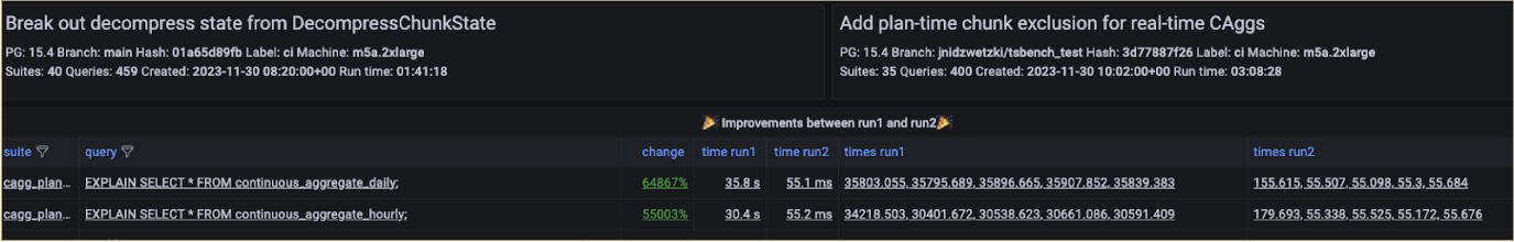
After constifying the watermark function call, we repeated our experiments with large continuous aggregates. We did our experiments on a hypertable consisting of 8,000 chunks to have a lot of chunks that could be covered by query planning. The results show a massive difference in the query time. The time for a SELECT query on the continuous aggregate (continuous_aggregate_hourly) went down from 33 seconds to 54 ms, a performance boost of 55,000 %.
We did the same SELECT query on a hierarchical continuous aggregate, which is defined on top of the first aggregate. The query on the hierarchical continuous aggregate (continuous_aggregate_daily) shows a similar performance boost. The time to execute the query went down from 35 seconds to 54 ms, which is a performance boost of 64,000 %.
Wrap-Up
In this blog post, we have discussed an optimization for real-time continuous aggregates in TimescaleDB 2.13.0. This enhancement reduces the PostgreSQL planning time immensely, with benchmarks showing that the total query execution time could be reduced by more than 50,000 %.
We made data aggregation faster by replacing the watermark function with a constant value. The watermark function returns the information up to which point a real-time continuous aggregate has to read data from the already pre-computed materialized hypertable and up to which part of the query needs to calculate the results on the fly. Using a constant value allows plan time chunk exclusion and plan scans only for the chunks that are actually accessed by the query.
To experience faster real-time data aggregations in PostgreSQL, along with other benefits, such as automatic data partitioning and storage savings via columnar compression, try TimescaleDB. You can create a free Timescale account or choose to host it yourself.