How to Analyze Cryptocurrency Market Data using TimescaleDB, PostgreSQL and Tableau: a Step-by-Step Tutorial

This tutorial is a step-by-step guide on how to analyze a time-series cryptocurrency dataset using Postgres, TimescaleDB and Tableau. The instructions in this tutorial were used to create this analysis of 4100+ cryptocurrencies.
Overview of steps
Step 0: Install TimescaleDB via Timescale Cloud: We’ll create a Timescale Cloud account and spin up a TimescaleDB instance.
Step 1: Design the database schema: We’ll guide you through how to design a schema for cryptocurrency data to use with TimescaleDB.
Step 2: Create a dataset to analyze: We’ll use the CryptoCompareAPI and Python to create a CSV file containing the data to analyze.
Step 3: Load dataset into TimescaleDB: We’ll insert the data from the CSV file into TimescaleDB using pgAdmin.
Step 4: Query the data in TimescaleDB: We’ll connect our data in TimescaleDB to Tableau and perform queries on the dataset.
Step 5: Visualize the results: We’ll use Tableau in order to visualize the results from our queries.
You can download all files and code used in this analysis in this Github repo. Note that the dataset provided tracks OHLCV price data on 4198 different cryptocurrencies (courtesy of CryptoCompare) as of 9/16/2019. Should you follow the steps correctly, your dataset will be up to the date that you perform the analysis.
Step 0: Install TimescaleDB via Timescale Cloud
Go to www.timescale.com/cloud and sign up for a free trial, where you will receive $300 in credits, to use a cloud-hosted and managed version of TimescaleDB. This is the easiest way to install the DB. If you prefer, you can install an instance yourself on your machine by following these instructions. However, the instructions in this post will assume you’re using Timescale Cloud.
After you’ve created an account, log-in and create a database instance (you can name it something like “crypto_database”). Then select your prefered configuration (dev-only should be enough for this analysis). After successfully creating the database instance, you should see it active.

Once the instance is active, navigate to “Databases” and create a new database. I’ve called mine ‘crypto-test’. You should see it in the list of Databases after its been created.

Step 1: Design the database schema
Now that our database is up and running we need some data to insert into it. Before we get data for analysis, we first need to define what kind of data we want to perform queries on. (To skip ahead, see the code in schema.sql)
In our analysis, we have two main goals.
- We want to explore the price of Bitcoin and Ethereum, expressed in different fiat currencies, over time.
- We want to explore the price of different cryptocurrencies, expressed in Bitcoin, over time.
Examples of questions we might want to ask are:
- How has Bitcoin’s price in USD varied over time?
- How has Ethereum’s price in ZAR varied over time?
- How has Bitcoin’s trading volume in KRW increased or decreased over time?
- Which crypto has highest trading volume in last two weeks?
- Which day was Bitcoin most profitable?
- Which are the most profitable new coins from the past 3 months?
Understanding the questions required of the data leads us to define a schema for our database, so that we can acquire the necessary data to populate it.
Our requirements leads us to 4 tables, specifically, three TimescaleDB hypertables, btc_prices, crypto_prices and eth_prices, and 1 relational table, currency_info.
The btc_prices hypertable contains data about Bitcoin prices in 17 different fiat currencies since 2010:
| btc_prices hypertable schema | |
|---|---|
| Field | Description |
| time | The day-specific timestamp of the price records, with time given as the default 00:00:00+00 |
| opening_price | The first price at which the coin was exchanged that day |
| highest_price | The highest price at which the coin was exchanged that day |
| lowest_price | The lowest price at which the coin was exchanged that day |
| closing_price | The last price at which the coin was exchanged that day |
| volume_btc | The volume exchanged in the cryptocurrency value that day, in BTC. |
| volume_currency | The volume exchanged in its converted value for that day, quoted in the corresponding fiat currency. |
| currency_code | Corresponds to the fiat currency used for non-btc prices/volumes. |
Similar to btc_prices, the eth_prices hypertable contains data about Ethereum prices in 17 different fiat currencies since 2015:
| eth_prices hypertable schema | |
|---|---|
| Field | Description |
| time | The day-specific timestamp of the price records, with time given as the default 00:00:00+00 |
| opening_price | The first price at which the coin was exchanged that day |
| highest_price | The highest price at which the coin was exchanged that day |
| lowest_price | The lowest price at which the coin was exchanged that day |
| closing_price | The last price at which the coin was exchanged that day |
| volume_eth | The volume exchanged in the cryptocurrency value that day, in ETH. |
| volume_currency | The volume exchanged in its converted value for that day, quoted in the corresponding fiat currency. |
| currency_code | Corresponds to the fiat currency used for non-ETH prices/volumes. |
The crypto_prices hypertable contains data about 4198 cryptocurrencies, including bitcoin and the corresponding crypto/BTC exchange rate, since 2012 or so.
| crypto_prices hypertable schema | |
|---|---|
| Field | Description |
| time | The day-specific timestamp of the price records, with time given as the default 00:00:00+00 |
| opening_price | The first price at which the coin was exchanged that day |
| highest_price | The highest price at which the coin was exchanged that day |
| lowest_price | The lowest price at which the coin was exchanged that day |
| closing_price | The last price at which the coin was exchanged that day |
| volume_eth | The volume exchanged in the cryptocurrency value that day, in ETH. |
| volume_currency | The volume exchanged in its converted value for that day, quoted in the corresponding fiat currency. |
| currency_code | Corresponds to the fiat currency used for non-ETH prices/volumes. |
Lastly, we have the currency_info hypertable, which maps the currency’s code to its name.
| currency_info table schema | |
|---|---|
| Field | Description |
| currency_code | 2-7 character abbreviation for currency. Used in other hypertables |
| currency | English name of currency |
Once we’ve established the schema for the tables in our database, we can formulate create_table SQL statements to actually create the tables we need:
Code from schema.sql:
--Schema for cryptocurrency analysis
DROP TABLE IF EXISTS "currency_info";
CREATE TABLE "currency_info"(
   currency_code   VARCHAR (10),
   currency        TEXT
);

--Schema for btc_prices table
DROP TABLE IF EXISTS "btc_prices";
CREATE TABLE "btc_prices"(
   time            TIMESTAMP WITH TIME ZONE NOT NULL,
   opening_price   DOUBLE PRECISION,
   highest_price   DOUBLE PRECISION,
   lowest_price    DOUBLE PRECISION,
   closing_price   DOUBLE PRECISION,
   volume_btc      DOUBLE PRECISION,
   volume_currency DOUBLE PRECISION,
   currency_code   VARCHAR (10)
);

--Schema for crypto_prices table
DROP TABLE IF EXISTS "crypto_prices";
CREATE TABLE "crypto_prices"(
   time            TIMESTAMP WITH TIME ZONE NOT NULL,
   opening_price   DOUBLE PRECISION,
   highest_price   DOUBLE PRECISION,
   lowest_price    DOUBLE PRECISION,
   closing_price   DOUBLE PRECISION,
   volume_crypto   DOUBLE PRECISION,
   volume_btc      DOUBLE PRECISION,
   currency_code   VARCHAR (10)
);

--Schema for eth_prices table
DROP TABLE IF EXISTS "eth_prices";
CREATE TABLE "eth_prices"(
   time            TIMESTAMP WITH TIME ZONE NOT NULL,
   opening_price   DOUBLE PRECISION,
   highest_price   DOUBLE PRECISION,
   lowest_price    DOUBLE PRECISION,
   closing_price   DOUBLE PRECISION,
   volume_eth      DOUBLE PRECISION,
   volume_currency DOUBLE PRECISION,
   currency_code   VARCHAR (10)
);

--Timescale specific statements to create hypertables for better performance
SELECT create_hypertable('btc_prices', 'time', 'opening_price', 2);
SELECT create_hypertable('eth_prices', 'time', 'opening_price', 2);
SELECT create_hypertable('crypto_prices', 'time', 'currency_code', 2);
Notice that we include 3 create_hypertable statements which are special TimescaleDB statements. For more on hypertables, see the Timescale docs and this blog post.
Step 2: Create a dataset to analyze
Now that we’ve defined the data we want, it’s time to construct a dataset containing that data. To do this, we’ll write a small python script (to skip ahead see crypto_data_extraction.py) for extracting data from cryptocompare.com into 4 csv files (coin_names.csv, crypto_prices.csv, btc_prices.csv and eth_prices.csv).
In order to get data from cryptocompare, you’ll need to obtain an API key. For this analysis, the free key should be plenty.
The script consists of 5 parts:
(1) Setup: First, we need to import some libraries to help us parse the data. Notably, we will use the python ‘requests’ library, which make it easy to deal with JSON data from a web API endpoint.
import requests
import json
import csv
from datetime import datetime
Moreover you’ll need your CryptoCompare API key as a variable. We’ve just included it as a normal variable in the code below (this is not recommended for production code) but you can store it as an environment variable or follow whatever production security practices for API key management you usually do.
apikey = 'YOUR_CRYPTO_COMPARE_API_KEY'
#attach to end of URLstring
url_api_part = '&api_key=' + apikey
(2) Get a list of all coin names to populate table currency_info: First we use the Python requests library’s get function to get a JSON object containing the list of coins names and symbols on CryptoCompare. Then we convert the data to a dictionary form and write information about the coin to the csv file ‘coin_names.csv’.
#####################################################################
#2. Populate list of all coin names
#####################################################################
#URL to get a list of coins from cryptocompare API
URLcoinslist = 'https://min-api.cryptocompare.com/data/all/coinlist'

#Get list of cryptos with their symbols
res1 = requests.get(URLcoinslist)
res1_json = res1.json()
data1 = res1_json['Data']
symbol_array = []
cryptoDict = dict(data1)

#write to CSV
with open('coin_names.csv', mode = 'w') as test_file:
   test_file_writer = csv.writer(test_file, delimiter = ',', quotechar = '"', quoting=csv.QUOTE_MINIMAL)
   for coin in cryptoDict.values():
       name = coin['Name']
       symbol = coin['Symbol']
       symbol_array.append(symbol)
       coin_name = coin['CoinName']
       full_name = coin['FullName']
       entry = [symbol, coin_name]
       test_file_writer.writerow(entry)
print('Done getting crypto names and symbols. See coin_names.csv for result')
(3) Get historical BTC prices for 4198 other cryptos to populate crypto_prices: Once we have the list of all the coin names, we can iterate through them and pull their historical prices in BTC since they listed on CryptoCompare. We write that information to the CSV file “crypto_prices.csv”.
#####################################################################
#3. Populate historical price for each crypto in BTC
#####################################################################
#Note: this part might take a while to run since we're populating data for 4k+ coins
#counter variable for progress made
progress = 0
num_cryptos = str(len(symbol_array))
for symbol in symbol_array:
   # get data for that currency
   URL = 'https://min-api.cryptocompare.com/data/histoday?fsym='+ symbol +'&tsym=BTC&allData=true' + url_api_part
   res = requests.get(URL)
   res_json = res.json()
   data = res_json['Data']
   # write required fields into csv
   with open('crypto_prices.csv', mode = 'a') as test_file:
       test_file_writer = csv.writer(test_file, delimiter = ',', quotechar = '"', quoting=csv.QUOTE_MINIMAL)
       for day in data:
           rawts = day['time']
           ts = datetime.utcfromtimestamp(rawts).strftime('%Y-%m-%d %H:%M:%S')
           o = day['open']
           h = day['high']
           l = day['low']
           c = day['close']
           vfrom = day['volumefrom']
           vto = day['volumeto']
           entry = [ts, o, h, l, c, vfrom, vto, symbol]
           test_file_writer.writerow(entry)
   progress = progress + 1
   print('Processed ' + str(symbol))
   print(str(progress) + ' currencies out of ' +  num_cryptos + ' written to csv')
print('Done getting price data for all coins. See crypto_prices.csv for result')
Notice how the fields defined in Step 1 influence the choice of what data we write to the CSV file!
(4) Get historical Bitcoin prices in different fiat currencies to populate btc_prices: We then create a list of different fiat currencies in which we want to express Bitcoin’s price. Unfortunately CryptoCompare doesn’t have a comprehensive list so we’ve hard coded (gasp!) a list of 17 popular fiat currencies.
We then iterate over the list of fiat currencies and pull the historical Bitcoin price in that currency and write it to the CSV file “btc_prices.csv”.
#####################################################################
#4. Populate BTC prices in different fiat currencies
#####################################################################
# List of fiat currencies we want to query
# You can expand this list, but CryptoCompare does not have
# a comprehensive fiat list on their site
fiatList = ['AUD', 'CAD', 'CNY', 'EUR', 'GBP', 'GOLD', 'HKD',
'ILS', 'INR', 'JPY', 'KRW', 'PLN', 'RUB', 'SGD', 'UAH', 'USD', 'ZAR']

#counter variable for progress made
progress2 = 0
for fiat in fiatList:
   # get data for bitcoin price in that fiat
   URL = 'https://min-api.cryptocompare.com/data/histoday?fsym=BTC&tsym='+fiat+'&allData=true' + url_api_part
   res = requests.get(URL)
   res_json = res.json()
   data = res_json['Data']
   # write required fields into csv
   with open('btc_prices.csv', mode = 'a') as test_file:
       test_file_writer = csv.writer(test_file, delimiter = ',', quotechar = '"', quoting=csv.QUOTE_MINIMAL)
       for day in data:
           rawts = day['time']
           ts = datetime.utcfromtimestamp(rawts).strftime('%Y-%m-%d %H:%M:%S')
           o = day['open']
           h = day['high']
           l = day['low']
           c = day['close']
           vfrom = day['volumefrom']
           vto = day['volumeto']
           entry = [ts, o, h, l, c, vfrom, vto, fiat]
           test_file_writer.writerow(entry)
   progress2 = progress2 + 1
   print('processed ' + str(fiat))
   print(str(progress2) + ' currencies out of  17 written')
print('Done getting price data for btc. See btc_prices.csv for result')
(5) Get historical Ethereum prices in different fiat currencies to populate eth_prices: Lastly, we do the same for Ethereum and the list of fiat currencies and write the results in the CSV file “eth_prices.csv”.
#####################################################################
#5. Populate ETH prices in different fiat currencies
#####################################################################
#counter variable for progress made
progress3 = 0
for fiat in fiatList:
   # get data for bitcoin price in that fiat
   URL = 'https://min-api.cryptocompare.com/data/histoday?fsym=ETH&tsym='+fiat+'&allData=true' + url_api_part
   res = requests.get(URL)
   res_json = res.json()
   data = res_json['Data']
   # write required fields into csv
   with open('eth_prices.csv', mode = 'a') as test_file:
       test_file_writer = csv.writer(test_file, delimiter = ',', quotechar = '"', quoting=csv.QUOTE_MINIMAL)
       for day in data:
           rawts = day['time']
           ts = datetime.utcfromtimestamp(rawts).strftime('%Y-%m-%d %H:%M:%S')
           o = day['open']
           h = day['high']
           l = day['low']
           c = day['close']
           vfrom = day['volumefrom']
           vto = day['volumeto']
           entry = [ts, o, h, l, c, vfrom, vto, fiat]
           test_file_writer.writerow(entry)
   progress3 = progress3 + 1
   print('processed ' + str(fiat))
   print(str(progress3) + ' currencies out of  17 written')
print('Done getting price data for eth. See eth_prices.csv for result')
If you’d rather not pull a fresh data set, you’re welcome to use the dataset we already created, but note that it only has data until 9/16/2019.
Step 3: Load dataset into TimescaleDB, using Timescale Cloud and pgAdmin
After following Step 2, you should have 4 CSV files (if not download them here).
The next step is to load this data into TimescaleDB in order to query it and perform our analysis. In Step 0, we created a TimescaleDB instance in Timescale Cloud, so all that’s left is to use pgAdmin to create the tables from Step 1 and transfer data from each csv file to the relevant table.
3.1 Connect to your TimescaleDB instance
Download and install pgAdmin, or your favorite postgres admin tool (utilities like psql also work). Once installed, login to your database using the credentials on the ‘Overview page’ of your Timescale Cloud instance as shown in Fig 3.

Once logged in, you should see something like Fig 4 below.

3.2 Use the SQL code from Step 1 to create tables
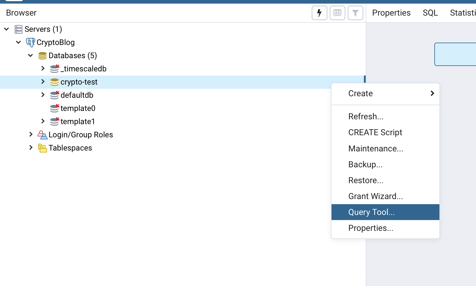
Now all our hard work in Step 1 comes in handy! Use the Query Tool in pgAdmin to create the tables we defined in Step 1. One way to find the tool is to navigate to your_project_name -> Databases-> your_db_name, then right click and select Query Tool, as Fig 5 shows below.
Next, we copy and paste the code from Step 1 (found in schema.sql) into the Query Editor and run the query. This creates the 4 tables with the necessary fields, as well as the 3 hypertables for btc_prices, eth_prices and crypto_prices.

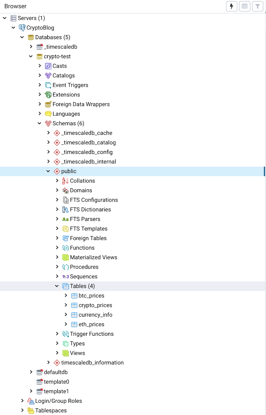
To check our query was successful, look at the output in the Data Output pane or navigate down to your_project_name -> databases-> your_db_name -> schemas -> tables and you should see your 4 tables.
3.3 Import the data into the database tables
Now that we’ve created the tables with our desired schema, all that’s left is to insert the data from the CSV files we’ve created into the tables.
We will do this using the Import tool in pgAdmin, but you could use psql or for better performance on large datasets, the TimescaleDB parallel-copy- tool. However, for files of the size we’ve created the pgAdmin import tool works just fine.
To import a CSV file to a table, navigate down to your_project_name -> databases-> your_db_name -> schemas -> tables and right click on the table you’d like to insert data into and then select ‘Import/Export’ from the menu, as shown in Fig 8 below. We’ll first insert data into the btc_prices table.

Once you’ve selected Import/Export, select Import, then select the csv file from your directory (in this case, btc_prices.csv), and then select comma (,) as the delimiter, as shown in Fig 9 below.

To check if this worked, right click on btc_prices table, select ‘view/edit data’ -> ‘all rows’, as shown in Fig 10. Fig 11 shows that our data has successfully been inserted into the btc_prices table.


Repeat these steps above for crypto_prices.csv and the crypto_prices table, eth_prices.csv and the eth_prices table and coin_names.csv and the currency_info table, respectively.
Step 4: Query the Data
With the data needed for our analysis now sitting snugly in our database tables, we can now perform queries on our dataset in order to answer some of the questions posed in Step 1.
The code below (from crypto_queries.sql) contains a sample list of questions and corresponding queries to answer those questions. Of course, you can add in your own questions and create Postgres queries to answer them in addition to, or in place of, the questions and queries provided.
From crypto_queries.sql:
-Query 1
-- How did Bitcoin price in USD vary over time?
-- BTC 7 day prices
SELECT time_bucket('7 days', time) as period,
      last(closing_price, time) AS last_closing_price
FROM btc_prices
WHERE currency_code = 'USD'
GROUP BY period
ORDER BY period

--Query 2
-- How did BTC daily returns vary over time?
-- Which days had the worst and best returns?
-- BTC daily return
SELECT time,
      closing_price / lead(closing_price) over prices AS daily_factor
FROM (
  SELECT time,
         closing_price
  FROM btc_prices
  WHERE currency_code = 'USD'
  GROUP BY 1,2
) sub window prices AS (ORDER BY time DESC)

--Query 3
-- How did the trading volume of Bitcoin vary over time in different fiat currencies?
-- BTC volume in different fiat in 7 day intervals
SELECT time_bucket('7 days', time) as period,
      currency_code,
      sum(volume_btc)
FROM btc_prices
GROUP BY currency_code, period
ORDER BY period

-- Q4
-- How did Ethereum (ETH) price in BTC vary over time?
-- ETH prices in BTC in 7 day intervals
SELECT
   time_bucket('7 days', time) AS time_period,
   last(closing_price, time) AS closing_price_btc
FROM crypto_prices
WHERE currency_code='ETH'
GROUP BY time_period
ORDER BY time_period

--Q5
-- How did ETH prices, in different fiat currencies, vary over time?
-- (using the BTC/Fiat exchange rate at the time)
-- ETH prices in fiat
SELECT time_bucket('7 days', c.time) AS time_period,
      last(c.closing_price, c.time) AS last_closing_price_in_btc,
      last(c.closing_price, c.time) * last(b.closing_price, c.time) FILTER (WHERE b.currency_code = 'USD') AS last_closing_price_in_usd,
      last(c.closing_price, c.time) * last(b.closing_price, c.time) FILTER (WHERE b.currency_code = 'EUR') AS last_closing_price_in_eur,
      last(c.closing_price, c.time) * last(b.closing_price, c.time) FILTER (WHERE b.currency_code = 'CNY') AS last_closing_price_in_cny,
      last(c.closing_price, c.time) * last(b.closing_price, c.time) FILTER (WHERE b.currency_code = 'JPY') AS last_closing_price_in_jpy,
      last(c.closing_price, c.time) * last(b.closing_price, c.time) FILTER (WHERE b.currency_code = 'KRW') AS last_closing_price_in_krw
FROM crypto_prices c
JOIN btc_prices b
   ON time_bucket('1 day', c.time) = time_bucket('1 day', b.time)
WHERE c.currency_code = 'ETH'
GROUP BY time_period
ORDER BY time_period

--Q6
--Crypto by date of first data
SELECT ci.currency_code, min(c.time)
FROM currency_info ci JOIN crypto_prices c ON ci.currency_code = c.currency_code
AND c.closing_price > 0
GROUP BY ci.currency_code
ORDER BY min(c.time) DESC

--Q7
-- Number of new cryptocurrencies by day
-- Which days had the most new cryptocurrencies added?
SELECT day, COUNT(code)
FROM (
  SELECT min(c.time) AS day, ci.currency_code AS code
  FROM currency_info ci JOIN crypto_prices c ON ci.currency_code = c.currency_code
  AND c.closing_price > 0
  GROUP BY ci.currency_code
  ORDER BY min(c.time)
)a
GROUP BY day
ORDER BY day DESC


--Q8
-- Which cryptocurrencies had the most transaction volume in the past 14 days?
--Crypto transaction volume during a certain time period
SELECT 'BTC' as currency_code,
       sum(b.volume_currency) as total_volume_in_usd
FROM btc_prices b
WHERE b.currency_code = 'USD'
AND now() - date(b.time) < INTERVAL '14 day'
GROUP BY b.currency_code
UNION
SELECT c.currency_code as currency_code,
       sum(c.volume_btc) * avg(b.closing_price) as total_volume_in_usd
FROM crypto_prices c JOIN btc_prices b ON date(c.time) = date(b.time)
WHERE c.volume_btc > 0
AND b.currency_code = 'USD'
AND now() - date(b.time) < INTERVAL '14 day'
AND now() - date(c.time) < INTERVAL '14 day'
GROUP BY c.currency_code
ORDER BY total_volume_in_usd DESC

--Q9
--Which cryptocurrencies had the top daily return?
--Top crypto by daily return
WITH
   prev_day_closing AS (
SELECT
   currency_code,
   time,
   closing_price,
   LEAD(closing_price) OVER (PARTITION BY currency_code ORDER BY TIME DESC) AS prev_day_closing_price
FROM
    crypto_prices
)
,    daily_factor AS (
SELECT
   currency_code,
   time,
   CASE WHEN prev_day_closing_price = 0 THEN 0 ELSE closing_price/prev_day_closing_price END AS daily_factor
FROM
   prev_day_closing
)
SELECT
   time,
   LAST(currency_code, daily_factor) as currency_code,
   MAX(daily_factor) as max_daily_factor
FROM
   daily_factor
GROUP BY
   TIME
For this step and in Step 5, we’ll use Tableau to run the above queries on the dataset and visualize the output. You’re welcome to use other data visualization tools like Grafana, but ensure that the tool you’ve selected has a Postgres connector.
The following steps are to query the data using Tableau:
4.1 Create a new workbook: This will be used to house all the graphs for the analysis.
4.2 Connect TimescaleDB to Tableau: Create a connection between Tableau and TimescaleDB running in your Timescale Cloud instance.
Connecting your TimescaleDB instance in the cloud to Tableau takes just a few clicks, thanks to Tableau’s built in Postgres connector. To connect to your database add a new connection and under the ‘to a server’ section, select PostgreSQL as the connection type. Then enter your database credentials (found in the Timescale Cloud ‘Overview’ tab) like we did in Step 3.

4.3 Create a new data source: Create a new datasource and rename it to be something unique, as by default it’s the name of your database.
You’ll need to do this for each query the analysis, since each data source only supports one piece of custom SQL. A way to create many data sources with the same database is to create one in the way described above, duplicate it and then change the custom SQL used each time, since the database you’re connecting to remains the same.
4.4 Query the data: Here we’ll use Tableau and the built in SQL editor. To run a query, add custom SQL to your data source by dragging and dropping the “New Custom SQL” button to the place that says ‘Add tables here’.

Once you’ve done that, paste the query you want in the query editor. In the example in Fig 14 below, we’ll use Query 1 from crypto_queries.sql, for historical BTC prices in USD.

Once you’ve entered the query, press OK and then Update Now and you’ll see the results in a table, as illustrated by Fig 15 below.

Step 5: Data Visualization in Tableau
Results in a table are only so useful, graphs are much better! So in our final step, let’s take our output from Step 4 and turn it into an interactive graph in Tableau.
To do this, create a new worksheet (or dashboard) and then select your desired data source (in our case ‘btc 7 days’), shown in Fig 16 below.

Next, you locate the Dimensions and Measures pane on the left.

Then, drag the period (time) dimension to ‘Columns’ part of sheet and then the ‘last closing price’ measure to the rows part of the worksheet. You should see something like the graph shown in Fig 18 below.

Now this graph doesn’t quite have the level of fidelity we’re looking for because the data points are being grouped by year. To fix this, click on the drop down arrow on period and select ‘exact date’.

This undoes the grouping by year and matches the price datapoint to the exact date that price occurred on. Your group should now look like Fig 20 below.

From there you can edit axis labels and colors and even add filter to zoom in on a specific time period. Here’s our final result, with labels added in Fig 21 below:

We encourage you to explore different visualization formats for the results you obtain from queries provided. For inspiration, check out the different visualizations we used in our analysis.
Conclusion
This tutorial showed you step by step one method of defining, creating, loading and analyzing a cryptocurrency market dataset. Here’s a reminder of what we covered:
- We created a Timescale Cloud account and spun up a TimescaleDB instance.
- We learned how to design a schema for cryptocurrency data for TimescaleDB and PostgreSQL.
- We used the CryptoCompareAPI and Python to create a CSV file containing the data to analyze
- We inserted the data from the CSV files created into TimescaleDB using pgAdmin and Timescale Cloud.
- We connected our data in TimescaleDB to Tableau and performed queries on the dataset
- We used Tableau to create graphs to visualize the results from our queries
Thank you for reading this far and if you followed all the steps, congratulations on successfully completing this tutorial! We hope you’ve enjoyed following along and that you’ve found this tutorial helpful.
Perhaps you’d also enjoy our analysis of over 4100 cryptocurrencies produced by following this tutorial.
For follow up questions or comments, reach out to us on Twitter (@TimescaleDB or @avthars), our community Slack channel, or reach out to me directly via email (avthar at timescale dot com).
Finally, if you’re interested in learning more about us, check out the Timescale website, Timescale Cloud, and see our GitHub and let us know how we can help!